In this example we will evaluate the shifted normal probability density function (the "bell-shaped curve") at equally spaced points and print the results using formatted printing with printf. We will also plot the points and demonstrate the use of several plot options, such as the use of title with titlefont, labels with labelfont, gridlines, etc.
Commands covered in this helpsheet:
restart ;
Digits := 16 ;
We will use 16 digit precision.
with(plots) :
| (1) |
| (2) |
| (3) |
| (4) |
| (5) |
 |
(6) |
The block ("do" loop) below:
printf("\n i x f (dec.form) f (sci. not.)\n" ) :
Click Shift+Enter
2) evaluates function f at each node x, and
3) prints the results in table form using formatted printing.
printf(" ---------------------------------------------------\n") :
Click Shift+Enter
for i from 0 to n do Click Shift+Enter
X[i] := a + i*h : Click Shift+Enter
Y[i] := f( X[i] ) : Click Shift+Enter
printf(" %5d %9.4f %13.9f %17.10e\n", i, X[i], Y[i], Y[i] ) :
Click Shift+Enter
end do:
i x f (dec.form) f (sci. not.)
---------------------------------------------------
0 60.0000 0.012238039 1.2238038602e-02
1 62.0000 0.047681764 4.7681764029e-02
2 64.0000 0.158309032 1.5830903166e-01
3 66.0000 0.447890606 4.4789060590e-01
4 68.0000 1.079819330 1.0798193303e+00
5 70.0000 2.218416694 2.2184166936e+00
6 72.0000 3.883721100 3.8837210997e+00
7 74.0000 5.793831055 5.7938310552e+00
8 76.0000 7.365402806 7.3654028061e+00
9 78.0000 7.978845608 7.9788456080e+00
10 80.0000 7.365402806 7.3654028061e+00
11 82.0000 5.793831055 5.7938310552e+00
12 84.0000 3.883721100 3.8837210997e+00
13 86.0000 2.218416694 2.2184166936e+00
14 88.0000 1.079819330 1.0798193303e+00
15 90.0000 0.447890606 4.4789060590e-01
16 92.0000 0.158309032 1.5830903166e-01
17 94.0000 0.047681764 4.7681764029e-02
18 96.0000 0.012238039 1.2238038602e-02
19 98.0000 0.002676605 2.6766045153e-03
20 100.0000 0.000498849 4.9884942580e-04
Notice how aesthetically pleasing and legible the output appears with the printf command.
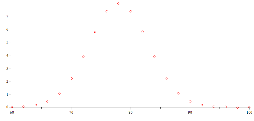
The following merely plots the points (X,Y) calculated above with no embellishment (no plot options). Notice that the plot is rather boring and nondescript.
plot( [ [X[k], Y[k]]$k = 0 .. n ], style = point ) ;
 |
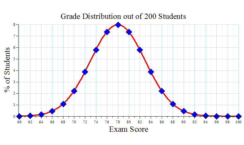
The following plots the
function f(x) as a curve
with more embellishment (with plot options) and stores the plot under name plot1.
Since we are storing the plot before displaying it, be sure to end the
command with a colon!
plot1 := plot( f(x), x = a .. b, 0. .. 8.0, thickness = 4, color = red,
Click Shift+Enter
title = "\n Grade Distribution out of 200 Students", titlefont = ["ROMAN", 20],
Click Shift+Enter
labelfont = ["ROMAN", 20], labels = ["Exam Score\n", "% of Students"],
Click Shift+Enter
labeldirections = ["horizontal", "vertical"],
Click Shift+Enter
axis[1] = [gridlines = [20, thickness = 1, subticks = true, color = "LightBlue"]],
Click Shift+Enter
axis[2] = [gridlines = [10, thickness = 1, subticks = false, color = "LightGray"]] ) :
The following plots the
function f(x) as discrete points with more embellishment and stores the plot under name plot2.
Again, be sure to end the command with a colon!
plot2 := plot( [ [X[k], Y[k] ]$k = 0 .. n ], style = point, symbol = soliddiamond, symbolsize = 24, color = blue) :
display( [ plot1, plot2 ] ) ; This displays both plots on a common graph.
 |
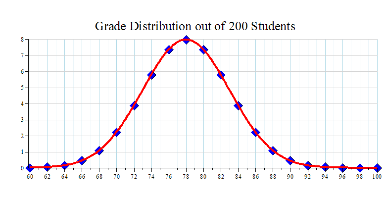
Notice what happens when you reverse the order of the plots in the display command:
display( [ plot2, plot1 ] ) ;
 |
Comments about some of the printf descriptors:
Example: %5d will print an integer up to
5 characters in length.
Example: %18.12f
W so that W ≥ D + 7.
Example: %19.12e
printf versus lprint
To appreciate the vast improvement produced by the printf command (to obtain formatted printing), let's see how the output appears when we use Maple's lprint command.
for i from 0 to n do Click Shift+Enter
X[i] := a + i*h : Click Shift+Enter
Y[i] := f( X[i] ) : Click Shift+Enter
lprint( i, X[i], Y[i], Y[i] ) :
Click Shift+Enter
end do:
0, 60.0, 0.1223803860227544e-1, 0.1223803860227544e-1
1, 62.00000000000000, 0.4768176402929684e-1, 0.4768176402929684e-1
2, 64.00000000000000, .1583090316595993, .1583090316595993
3, 66.00000000000000, .4478906058968579, .4478906058968579
4, 68.00000000000000, 1.079819330263761, 1.079819330263761
5, 70.00000000000000, 2.218416693589111, 2.218416693589111
6, 72.00000000000000, 3.883721099664259, 3.883721099664259
7, 74.00000000000000, 5.793831055229654, 5.793831055229654
8, 76.00000000000000, 7.365402806066466, 7.365402806066466
9, 78.00000000000000, 7.978845608028653, 7.978845608028653
10, 80.00000000000000, 7.365402806066466, 7.365402806066466
11, 82.00000000000000, 5.793831055229654, 5.793831055229654
12, 84.00000000000000, 3.883721099664259, 3.883721099664259
13, 86.00000000000000, 2.218416693589111, 2.218416693589111
14, 88.00000000000000, 1.079819330263761, 1.079819330263761
15, 90.00000000000000, .4478906058968579, .4478906058968579
16, 92.00000000000000, .1583090316595993, .1583090316595993
17, 94.00000000000000, 0.4768176402929684e-1, 0.4768176402929684e-1
18, 96.00000000000000, 0.1223803860227544e-1, 0.1223803860227544e-1
19, 98.00000000000000, 0.2676604515297707e-2, 0.2676604515297707e-2
20, 100.0000000000000, 0.4988494258010713e-3, 0.4988494258010713e-3
Notice how unwieldy, objectionable,
unappealing, and misaligned
the output appears with the lprint command.
The printf command gives much more comprehensible and legible output.