Dr. Kevin G. TeBeest
Assoc. Prof. of Applied Mathematics
Kettering University

Example 5:  Forced Motion with Transient and Steady State Terms

>	de := 2*diff(x(t),t$2) + 24*diff(x(t),t) + 272*x(t) = 1200*sin(8*t);

(1)

Solve the above ODE, subject to initial conditions x(0) = 4  and  x'(0) = 36 . Store the result in X:

>	X := rhs( dsolve( {de, x(0) = 4, D(x)(0) = 36 }, x(t) ) );

(2)

Simplify the solution, and store the result in X:

>	X := combine( X, trig );

(3)

>	xp := -4*cos(8*t) + 3*sin(8*t);

(4)

 

Plot the solution: 

>	plot( [ xp, X ], t = 0 .. 2, thickness = [10, 5], color = [red, blue], title = `Ex 5: Forced Motion`, ytickmarks = 5, thickness = 5, titlefont = [HELVETICA, BOLD, 16], legend = ["Partic. Soln xp(t)     ", "Solution x(t)"], legendstyle = [ font = [HELVETICA,BOLD,14] ], size = [560,400] );

 

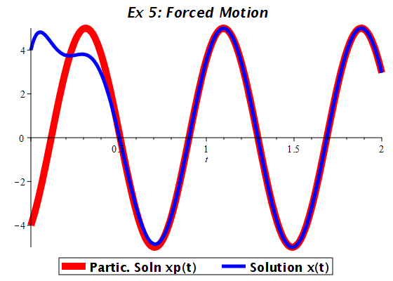The complementary solution x_c(t) represents decaying oscillation while the particular solution x_p(t) is simple harmonic. In this case we say the complementary solution is transient and the particular solution is steady. So after a sufficient amount of time has passed (about 1/2 second in this example), the motion has reached steady state, and we may approximate the equation of motion x(t) by the particular solution.