Plotting in Polar Coordinates

Dr. K. G. TeBeest

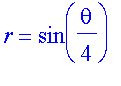
Example 8: Plot

Note how the curve fills in as the range is increased.

Here is used instead of since is easier to type.

> r:= sin( t / 4 );

> plot( r, t = 0 .. 1*Pi/2, coords = polar, scaling = constrained, thickness = 2);

> plot( r, t = 0 .. 2*Pi/2, coords = polar, scaling = constrained, thickness = 2);

> plot( r, t = 0 .. 3*Pi/2, coords = polar, scaling = constrained, thickness = 2);

> plot( r, t = 0 .. 4*Pi/2, coords = polar, scaling = constrained, thickness = 2);

> plot( r, t = 0 .. 5*Pi/2, coords = polar, scaling = constrained, thickness = 2);

> plot( r, t = 0 .. 6*Pi/2, coords = polar, scaling = constrained, thickness = 2);

> plot( r, t = 0 .. 7*Pi/2, coords = polar, scaling = constrained, thickness = 2);

> plot( r, t = 0 .. 8*Pi/2, coords = polar, scaling = constrained, thickness = 2);

> plot( r, t = 0 .. 9*Pi/2, coords = polar, scaling = constrained, thickness = 2);

> plot( r, t = 0 .. 9*Pi/2, coords = polar, scaling = constrained, thickness = 2);

> plot( r, t = 0 .. 10*Pi/2, coords = polar, scaling = constrained, thickness = 2);

> plot( r, t = 0 .. 11*Pi/2, coords = polar, scaling = constrained, thickness = 2);

> plot( r, t = 0 .. 12*Pi/2, coords = polar, scaling = constrained, thickness = 2);

> plot( r, t = 0 .. 13*Pi/2, coords = polar, scaling = constrained, thickness = 2);

> plot( r, t = 0 .. 14*Pi/2, coords = polar, scaling = constrained, thickness = 2);

> plot( r, t = 0 .. 15*Pi/2, coords = polar, scaling = constrained, thickness = 2);

> plot( r, t = 0 .. 16*Pi/2, coords = polar, scaling = constrained, thickness = 2);