FORMATTED PRINTING AND PLOT OPTIONS

Using Formatted Printing and Various Plot Options 

In this example we will evaluate the shifted normal probability density function (the "bell-shaped curve") at equally spaced points
and print the results using formatted printing with the printf command. We will also plot the points and demonstrate the use of
several plot options, such as the use of title with titlefont, labels with labelfont, gridlines, etc. 

Commands covered in this helpsheet:

I recommend beginning each Maple session with restart. When making any changes in your worksheet, it is wise to start here by clicking the restart command.

restart ;
Digits := 16 ;   We will use 16 digit precision arithmetic. Maple's default is 10 digit arithmetic.

(1)

with(plots) :     This loads some special plot options.  

(2)

(3)

(4)

(5)

(6)

The block ("do" loop) below:

printf("\n    i        x       f (dec.form)    f (sci. notat.)\n" ) :   Click Shift+Enter
printf("  ---------------------------------------------------\n") :     Click Shift+Enter
for i from 0 to n do     Click Shift+Enter
   X[i] := a + i*h :     Click Shift+Enter
   Y[i] := f( X[i] ) :   Click Shift+Enter
   printf(" %5d  %9.4f  %13.9f   %17.10e\n", i, X[i], Y[i], Y[i] ) :    Click Shift+Enter
end do :

i        x       f (dec.form)    f (sci. notat.)  ---------------------------------------------------     0    60.0000    0.012238039    1.2238038602e-02     1    62.0000    0.047681764    4.7681764029e-02     2    64.0000    0.158309032    1.5830903166e-01     3    66.0000    0.447890606    4.4789060590e-01     4    68.0000    1.079819330    1.0798193303e+00     5    70.0000    2.218416694    2.2184166936e+00     6    72.0000    3.883721100    3.8837210997e+00     7    74.0000    5.793831055    5.7938310552e+00     8    76.0000    7.365402806    7.3654028061e+00     9    78.0000    7.978845608    7.9788456080e+00    10    80.0000    7.365402806    7.3654028061e+00    11    82.0000    5.793831055    5.7938310552e+00    12    84.0000    3.883721100    3.8837210997e+00    13    86.0000    2.218416694    2.2184166936e+00    14    88.0000    1.079819330    1.0798193303e+00    15    90.0000    0.447890606    4.4789060590e-01    16    92.0000    0.158309032    1.5830903166e-01    17    94.0000    0.047681764    4.7681764029e-02    18    96.0000    0.012238039    1.2238038602e-02    19    98.0000    0.002676605    2.6766045153e-03    20   100.0000    0.000498849    4.9884942580e-04

Notice how tidy and legible the output appears with the printf command.
The output appears in column format and all decimals are properly aligned.
The printf format descriptors are explained below.

Plotting

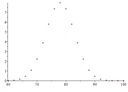
The following command merely plots the points (X,Y) calculated above with no embellishment (no plot options).
Notice that the plot is boring, nondescript, and even difficult to see, ESPECIALLY when printed on paper. 

plot( [ [X[k], Y[k]]$k = 0 .. n ], style = point, size = [500, 360] ) ; 

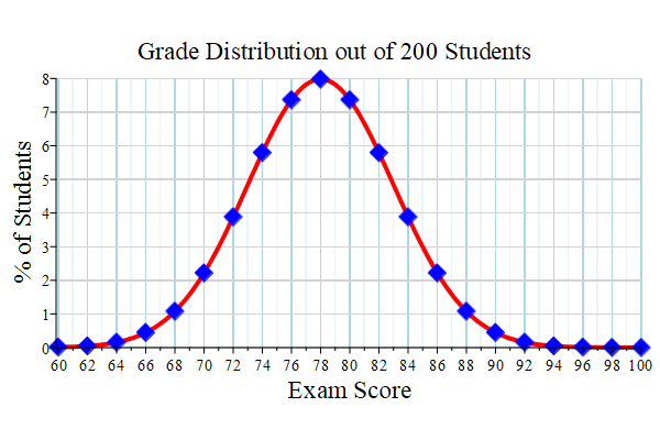
The following set of 6 lines creates a plot of the same function f(x) above but as a curve with much more embellishment (using plot options) and stores the plot under name plot1.
Since we are storing the plot before displaying it, be sure to end the command with a colon!

plot1 := plot( f(x), x = a .. b, 0.0 .. 8.0, thickness = 4, color = red, size = [600, 400],    Click Shift+Enter
title = "\n Grade Distribution out of 200 Students", titlefont = ["ROMAN", 20],    Click Shift+Enter
labelfont = ["ROMAN", 20], labels = ["Exam Score\n", "% of Students"],    Click Shift+Enter
labeldirections = ["horizontal", "vertical"],    Click Shift+Enter
axis[1] = [gridlines = [20, thickness = 1, subticks = true, color = "LightBlue"]],    Click Shift+Enter
axis[2] = [gridlines = [10, thickness = 1, subticks = false, color = "LightGray"]] ) :

The following creates a plot of the same function f(x) as discrete points with more embellishment and stores the plot under name plot2.
Again, be sure to end the command with a colon!

plot2 := plot( [ [X[k], Y[k] ]$k = 0 .. n ], style = point, symbol = soliddiamond, symbolsize = 24, color = blue, size = [600, 400]) : 

display( [ plot1, plot2 ] ) ;    This displays both plot1 and plot2 on a common graph.

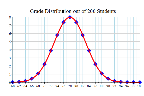
Notice what happens when we reverse the order of the plots in the display command:

display( [ plot2, plot1 ] ) ;

printf   versus  lprint

To appreciate the superiority of the printf command (to obtain formatted printing), let's see how the output appears when we use Maple's basic lprint command.

for i from 0 to n do     Click Shift+Enter
   X[i] := a + i*h :     Click Shift+Enter
   Y[i] := f( X[i] ) :   Click Shift+Enter
   lprint( i, X[i], Y[i], Y[i] ) :   Click Shift+Enter
end do:

0,60.0,0.1223803860227544e-1,0.1223803860227544e-1
1,62.00000000000000,0.4768176402929684e-1,0.4768176402929684e-1
2,64.00000000000000,.1583090316595993,.1583090316595993
3,66.00000000000000,.4478906058968579,.4478906058968579
4,68.00000000000000,1.079819330263761,1.079819330263761
5,70.00000000000000,2.218416693589111,2.218416693589111
6,72.00000000000000,3.883721099664259,3.883721099664259
7,74.00000000000000,5.793831055229654,5.793831055229654
8,76.00000000000000,7.365402806066466,7.365402806066466
9,78.00000000000000,7.978845608028653,7.978845608028653
10,80.00000000000000,7.365402806066466,7.365402806066466
11,82.00000000000000,5.793831055229654,5.793831055229654
12,84.00000000000000,3.883721099664259,3.883721099664259
13,86.00000000000000,2.218416693589111,2.218416693589111
14,88.00000000000000,1.079819330263761,1.079819330263761
15,90.00000000000000,.4478906058968579,.4478906058968579
16,92.00000000000000,.1583090316595993,.1583090316595993
17,94.00000000000000,0.4768176402929684e-1,0.4768176402929684e-1
18,96.00000000000000,0.1223803860227544e-1,0.1223803860227544e-1
19,98.00000000000000,0.2676604515297707e-2,0.2676604515297707e-2
20,100.0000000000000,0.4988494258010713e-3,0.4988494258010713e-3

Notice how unwieldy, untidy, misaligned, tacky, clumsy, inelegant, unrefined, crude, unpleasant, disagreeable, obnoxious, nauseating, unappealing, objectionable, disgusting, vulgar, hideous, repulsive, and excruciatingly grotesque the output appears with the lprint command. One column is screaming: "Why are you printing all those trailing zeros? Isn't that a bit redundant?!?!"
When would the lprint command ever be used? When you might want a comma delimited (csv) file.

The printf command gives much more comprehensible and legible output.
When printf is used CORRECTLY,

1. columns should align,
2. decimal points in a given column should always line up,
3. the right-most digit of integers in a given column should align,
4. decimal numbers that are expected to be very small or very large should be printed in scientific notation,
5. decimal numbers that are expected to be moderate in size should be printed in decimal form, and
6. table headers should be used for each column and should be CENTERED above their respective columns.